This comes from a talk I’m giving at Penguicon 2012. The talk in general is about weight loss and getting healthy but part of it involves doing some predictive modeling of future weights based on calorie counting.
Consider the question “if I eat X number of calories a day, will I gain or lose weight?”. It’s a supremely practical question but without doing some research it isn’t immediately apparent how to answer this. The best place to start is one of the formulas for calculating basal metabolic rate. The obligatory Wikipedia link provides some more background but in short it gives us a formula for the “baseline” number of calories our body needs. Mifflin-St. Jeor is considered by many [citation needed] to be the most accurate. It is of the form:
In this formula, m is mass in kilograms, h is height in centimeters, a is age in years, and s is a gender offset which is either +5 for men or -161 for women. This gives us P, our basal metabolic rate in calories. An interesting thing about BMR is that it’s a measure of your caloric needs at more or less complete rest. A normal person’s caloric needs to maintain weight will usually be strictly greater than their BMR. Because of this, P is usually scaled by an “activity factor” which factors in daily life. This can range from ~1.2 for someone with a desk job who gets no exercise to ~1.9 for someone who engages in some serious workouts. Now that we know our caloric needs, how can use this to model where our weight will be in the future?
Let’s modify the M-SJ equation to use some arbitrary function w(t) which gives our weight after time t instead of the constant m. I’ll also bring in the activity factor f. Now we have:
An apology to my metric-inclined friends but I’m using w(t)‘s output as pounds (which is why I’m dividing by 11/5 to convert to kilograms). P is now our adjusted metabolic rate. Let’s insert a new variable, d, which will represent our daily diet in calories. If we take d and subtract it by P, we will have our daily net caloric deficit/surplus.
It’s an accepted estimate that 3500 calories equals one pound. If we divide this whole equation by 3500, we’ll have how much we’d expect to our weight to change by eating d calories when weighing w(t). But, this is precisely the derivative of w(t)! Our equation now looks something like this:
This allows us to solve for w(t).
The left term is the weight we’re asymptotic to; our “plateau”. c1 is the constant of integration. At t = 0, w(t) equals the left term plus c1. To model for a specific person, t = 0 should be equal to their starting weight. Therefore, c1 should be equal to the difference between their start weight and the left term.
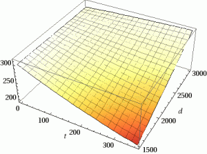
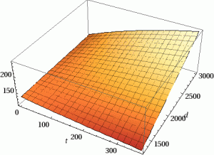
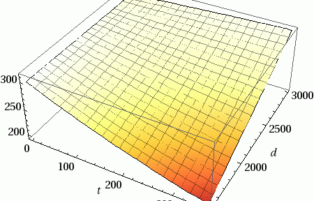
We’ve created a nice complicated formula, but sadly this a 7-dimensional surface (8 if you include the starting weight) and doesn’t offer much in the way of visualization. To get some more concrete results. Let’s pick some values for the constants a, h, s, f and starting weight which are invariant (more or less) for a given person.


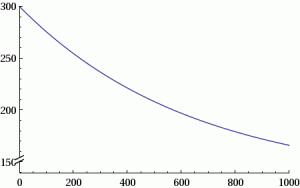
Pretty 3D! If we pick a fixed diet d the graph becomes even more instructional.

Hope this was insightful! For anyone in the Metro Detroit area, I’ll be speaking more on this again at Penguicon 2012. See you there!
This work is licensed under a Creative Commons Attribution-ShareAlike 4.0 International License.


Leave a Reply